Page contents
How do I find the operating point of a pump on its system?
The operating point is the intersection of two curves: the pump curve, head H against flow rate Q, supplied by the manufacturer, and the system curve, Hsystem = Hs + k × Q², the sum of the static head Hs to overcome and of the head losses, which grow as the square of the flow rate. The pump settles by itself at the flow rate where both heads are equal. Example: a pump with the curve H = 30 − 0.1 Q² (Q in m³/h, H in m) on a system with 10 m of static head and 5 m of losses at 10 m³/h (k = 0.05): the equality 30 − 0.1 Q² = 10 + 0.05 Q² gives Q = 11.5 m³/h and H = 16.7 m, i.e. a hydraulic power ρ g Q H of 524 W and 873 W absorbed at an efficiency of 60 %. The calculator below plots your pump curve from the catalogue points and your system curve, and finds their intersection, the power and the case of pumps in series or in parallel.
Operating point formulas
- Hpump: head of the pump, in m of the pumped liquid, read on the manufacturer's curve; it falls as the flow rate rises
- Hs: static head, in m, level difference between the suction and discharge free surfaces (plus tank pressures converted to m); zero in a closed circuit
- k × Q²: head losses of the system, in m; k follows from the losses ΔH₀ calculated at one flow rate Q₀ (for instance with the head loss calculator)
- Q: flow rate, in m³/s in the power formulas (1 m³/h = 1/3,600 m³/s); ρ: density in kg/m³; g = 9.81 m/s²
- Phyd: useful hydraulic power, in W; Pshaft: power absorbed on the shaft, η pump efficiency (0.4 to 0.8)
Finding the operating point: worked example
| Flow rate Q | Pump head H | Head required by the system | Situation |
|---|---|---|---|
| 0 m³/h | 30.0 m | 10.0 m | valve closed: the pump supplies more than needed |
| 4 m³/h | 28.4 m | 10.8 m | the pump has spare head, the flow rate increases |
| 8 m³/h | 23.6 m | 13.2 m | same |
| 11.5 m³/h | 16.7 m | 16.7 m | operating point |
| 12 m³/h | 15.6 m | 17.2 m | the pump can no longer supply the required head |
| 16 m³/h | 4.4 m | 22.8 m | impossible |
Shift of the operating point when the system changes
| System | Operating point | Hydraulic power | Shaft power |
|---|---|---|---|
| Initial system: Hs = 10 m, k = 0.05 | 11.5 m³/h, 16.7 m | 524 W | 873 W |
| Valve partly closed: k doubled (0.10) | 10.0 m³/h, 20.0 m | 544 W | 907 W |
| Static head raised to 15 m, k = 0.05 | 10.0 m³/h, 20.0 m | 544 W | 907 W |
| Closed circuit: Hs = 0, k = 0.05 | 14.1 m³/h, 10.0 m | 385 W | 641 W |
Detailed explanations and calculation in Mecaflux
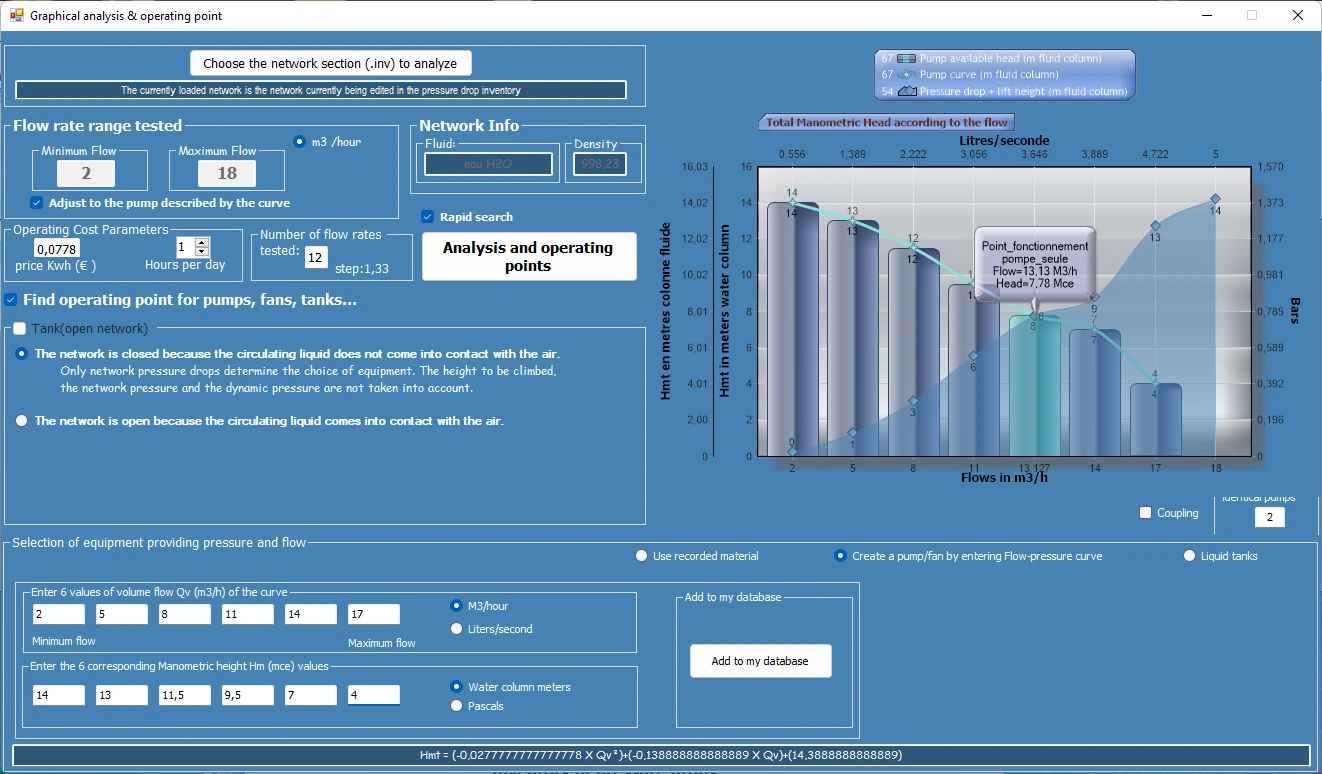
The pump operating point pumps is discussed in the page pumps, we see here an example of calculation of the operating point of the pump, This is similar to ventilations or apiration (with no control of NPSH because no risk of cavitation with the air).The flow rate that delivers a centrifugal pump or fan decreases depending on the pressure resistant (load height or Delta pressure) of the fluid's network. This resistance of the network is the pressure that must provide the pump or fan, to achieve a given rate.
the manufacturer provides with the pump, a flow curve of evolution, as a function of the pressure resistant, that the pump has to overcome.. The curves are generally provided for a family of pump. Pressure (or delta P for the fans), is given in Hm (manometric head) for liquids, or Pascals for aeraulic.
- As a simple reminder, 1 meter water column produces a pressure (Density X Gravity X Height) 1000 x 9,81 x 1 = 9810 pascals. 1 bar=100 000 pascals we note that 1 bar = 10 water meters = 100 000 pascals
Pump wheel diameter reduced: In theory the flow and manometric head are proportional to the square of the diameter of the wheel. wheel diameter reduced is used to modify the pump flow without modifying its performance, (in a limit of 15% of the initial diameter), This therefore gives the possibility to manufacturer, to using a model of pump to produce a range of pumps perfectly adapted to various specifications.
We see for example that the pump with wheel 116 mm provides a pressure of 110 Meters, to flow rate of 2 m3 /h in its area of best efficiency (about 42% ). Here we can read the graph of the pump, It remains to see if it corresponds to our network. The question that arises is: What is the pressure required to circulate the fluid in our system, to the flow rate that we want to achieve? At the flow rate that we want to achieve, the pressure provided by the pump must be equal to the sum of:- head loss (friction losses and turbulence in the conduct constituting the system and Accessories. See major head loss and minor head loss))
- static pressure: Height difference between the point of input and output circuit (zero if the network is closed. See hydrostatic head)
- Dynamic pressure: acceleration of the fluid, it is the kinetic-energy (speed) supplied to the fluid.
- The operating point of the system "pump / network" is the flow rate that balances the pressure supplied by the pump and pressure necessary for the operation of the network flow.
- The yellow curve intersects the curve network, to operating point 3 m³/h
- The dark blue curve intersects the curve network, to operating point 2,2 m³/h
- The red curve pump is outside the range of flow in which the network was tested (light blue curve) But we can imagine that if the curve network continues to evolve in this way, it crosses the red line at the operating point of 3,5 m³/h
Another example video:
Frequently asked questions
What happens when a discharge valve is partly closed?
The system curve steepens (k increases) and the operating point moves up along the pump curve: the flow rate drops, the head rises. In the example, doubling k brings the flow rate from 11.5 to 10 m³/h and the head from 16.7 to 20 m. It is a simple way to set the flow rate of a centrifugal pump, but the energy dissipated in the valve is lost; a variable speed drive, which lowers the pump curve, is more economical. Close to the shut-off point the efficiency collapses and the pump heats up.
How do I find the operating point of pumps in series or in parallel?
Two identical pumps in series add their heads at equal flow rate (curve twice as high); in parallel they add their flow rates at equal head (curve twice as wide). The operating point is the intersection of this combined curve with the system curve: since the system resists more as the flow rate rises, two pumps in parallel always give less than twice the flow rate of one, and all the less as the system is steep. The calculator above handles both arrangements.
Why does the static head vanish in a closed circuit, and what about a fan?
In a closed circuit (heating, cooling) the liquid rising in one branch comes back down in the other: the columns balance out and the pump only has the head losses to overcome, so the system curve passes through the origin. For a fan the reasoning is the same with pressures in pascals: convert them into metres of air (ΔP / (ρ g), with ρ = 1.2 kg/m³, 100 Pa are worth 8.5 m of air) or use the curves in pascals of Mecaflux directly.
How do I determine the operating point of my own pump on my installation?
The pump editor of Mecaflux Standard stores the curves of your pumps entered from the catalogue, then the software crosses them with the system curve it has calculated section by section: operating point, power, efficiency and available NPSH are displayed, with a warning in case of cavitation. For a complete pumping installation to design or check, Mecaflux carries out the study of your project and delivers the calculation report, or offers training on the software applied to your own installation.